Main takeaways:
- The analysis below tries to identify real and financial shocks in the economy.
- It then looks at some of the recent financial shocks (the 6 largest shocks since 1990) to evaluate their impact on economic activity.
- The conclusion is that a median financial shock would reduce GDP growth to around 0.7%-1.2% range by early 2016.
- The median financial shock is similar to LTCM, WorldCom, 9/11 -- the current one does not feel as bad; however, the financial variables (volatility, spreads, etc.) are behaving as if it was.
- Taking at face value (and assuming the level of stress in the mkt continues), the current episode would be worse than the median financial shock (current episode means prices of last Wednesday).
- Note: the above simulations do not consider the impact of lower oil prices:
- First quarter growth hinted at a negative effect, as investment in the oil sector collapsed and the consumer did not pick up the tab.
- However, most of the hit on investment is behind (rigs counts turned positive by mid-July and have kept that way until end of Aug).
- More analysis is needed.
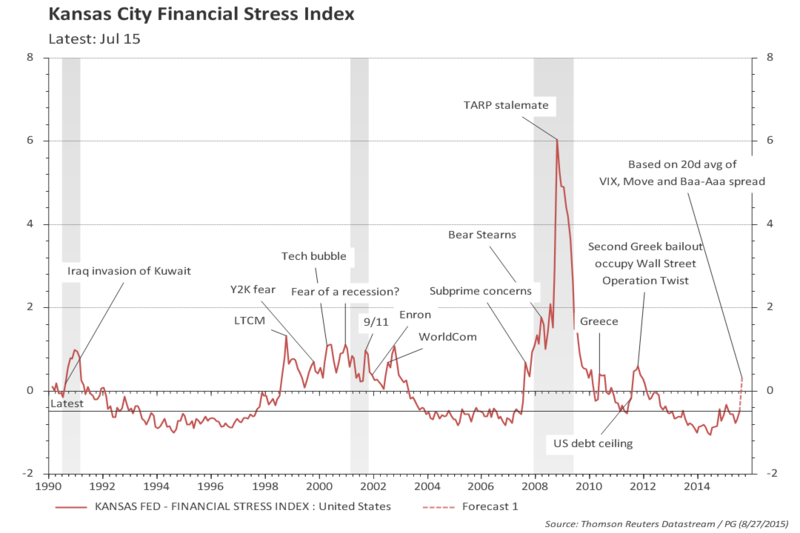
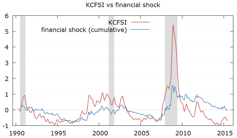
The KCFSI is calculated to have zero mean and 1 standard deviation. It has not yet been updated for the month of August, but based on measures of VIX, MOVE, and Baa-Aaa spread, one can infer the last 20d average at 0.3 (i.e., 0.3 standard deviation). Based only on August 26 data, the KCFSI would be closer to or slightly above one standard deviation -- a level reached during the crisis of late 1998 to 2002 period (LTCM, 9/11, WorldCom, etc.)
VAR model
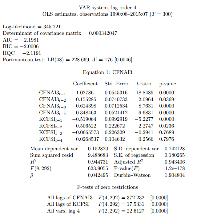
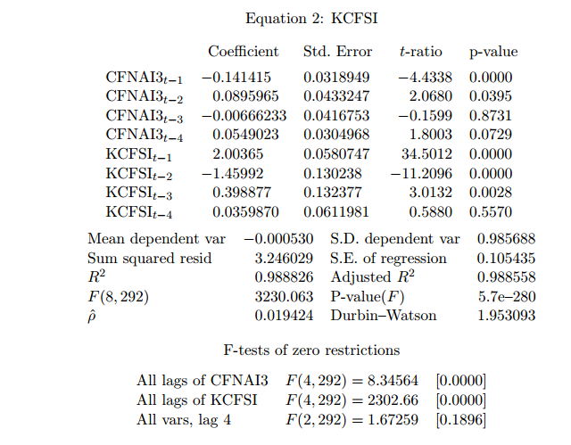
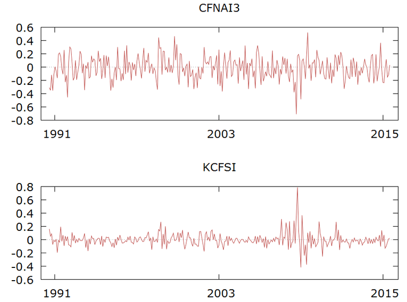
The residuals from the VAR are the actual (real and financial) shocks. They are clearly stationary and close to being white-noise.
In order to better understand the dynamics of the financial shocks, I will add the residuals cumulatively. In that way, a sequence of positive residuals (shocks) will not cancel out and will show as an increase in the cumulative financial shock hitting the economy.
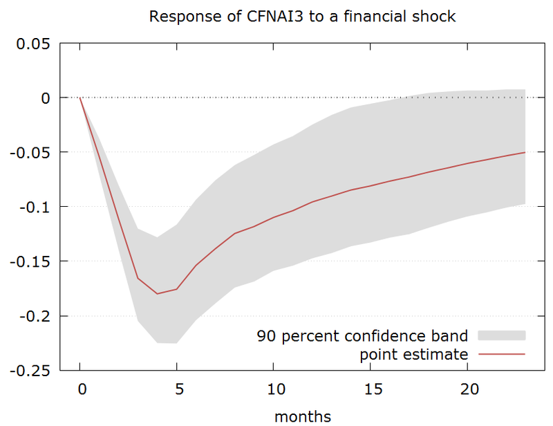
The standard deviation of the financial shock is around 0.1 -- and the chart below shows the impact of a one standard deviation financial shock into the economic activity (as measured by the CFNAI): it has a peak impact of around 3 to 5 months and reduces the CFNAI by 0.18 (from the baseline of no shock) in this period.
However, there is often periods where the financial shocks happen in sequence. In order to see that one can look at periods where the cumulative financial shock is increasing. There are a few of these periods since 1990.
But what about the oil shock? Is it positive or negative?
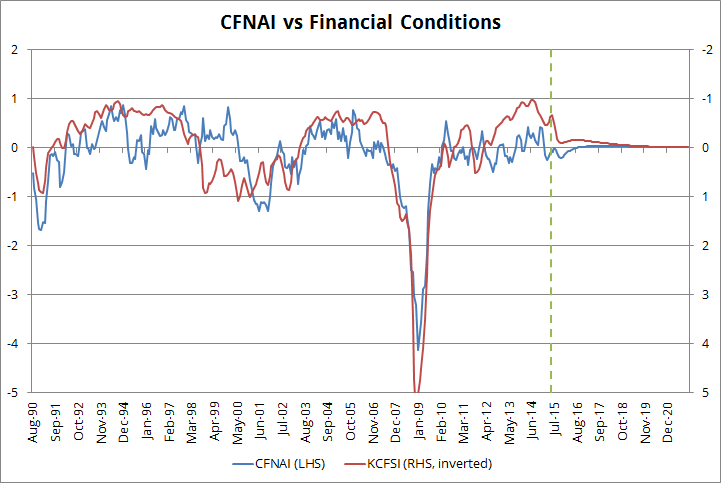
One useful measure of economic activity / growth is the Chicago Fed National Activity Index (CFNAI) - see Filtering US GDP noise using CFNAI.
How can one infer the size of a financial shock from the KCFSI (or from any other FCI or FSI)?
One could argue that if the KCFCI moved from, say, -0.2 in a given month (t=0) to 0.3 in the following month (t=1), then there was a financial shock of around 0.5 standard deviation. However, this is not accurate since the time series for the index has a large degree of persistence (memory). As a matter of fact, there is a high likelihood that the financial conditions index would increase further in t=2, and it would not be appropriate to attribute the increase in t=2 to a new financial shock -- it would be considered a follow through from the shock that had occurred in t=0.
What about the size of a shock to real economic activity?
A similar reasoning would apply. Moreover, it would also be important to disentangle the shock to economic activity coming from the financial shock and the one coming from the real shock.
So, what should one do?
A simple alternative is to estimate a VAR model (vector autoregression). Doing that (after checking for the appropriated lags, for the stationarity of residuals, for autocorrelation in the residuals, etc.) I obtain:
VAR model
The residuals from the VAR are the actual (real and financial) shocks. They are clearly stationary and close to being white-noise.
In order to better understand the dynamics of the financial shocks, I will add the residuals cumulatively. In that way, a sequence of positive residuals (shocks) will not cancel out and will show as an increase in the cumulative financial shock hitting the economy.
The chart below makes this point clear: the KCFSI measures the level of financial conditions / stress, while the cumulative financial shock measures the cumulative effects of the new financial shocks into the economy. Both series are similar, but there are some interesting differences. For instance, in the period from 2004 to 2007 the KCFSI remained relatively stable, while the cumulative financial shock was trending down, showing that the economy had been consistently hit by positive new financial shocks.
The standard deviation of the financial shock is around 0.1 -- and the chart below shows the impact of a one standard deviation financial shock into the economic activity (as measured by the CFNAI): it has a peak impact of around 3 to 5 months and reduces the CFNAI by 0.18 (from the baseline of no shock) in this period.
The rule of thumb to translate CFNAI to GDP is each 0.1 in CFNAI is equivalent to 0.25pp in underlying growth. Therefore the impact of a one standard deviation shock in financial conditions to growth would be to cut growth by around -0.5pp 3 to 5 months down the road.
In the sample period from 1990 only 10% of the financial shocks were above 0.10 -- so the above calculation is representative of a really bad outcome.
However, there is often periods where the financial shocks happen in sequence. In order to see that one can look at periods where the cumulative financial shock is increasing. There are a few of these periods since 1990.
A more realistic scenario, perhaps, would be to replicate the previous cycles of a sequence of financial shocks.
There are 6 episodes where the cumulative financial shock over a 6-month period reached above 0.4: Feb/99, May/00, Sep/02, Jan/08, Dec/08, and Oct/11.
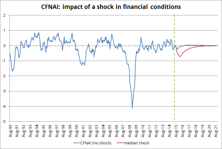
In the absence of shocks, both the CFNAI and the financial conditions KCFSI will converge to their equilibria in the long run, as shown in the chart below (zero CFNAI is equivalent to GDP growing at 2.5%):
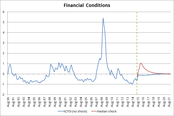
If I assume no shock on the real economy (no shock to CFNAI) and a median shock for financial conditions (median from the above mentioned episodes) it results in the following:
a) a hit to financial conditions similar to the ones observed in the 1998-2002 period.
b) CFNAI dropping to -0.7; this would be equivalent to GDP growing at 0.7% by early 2016.
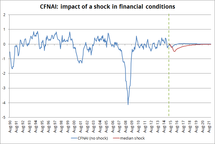
An alternative simulation would consider likely shocks to real economic activity (CFNAI) instead of assuming them zero. Using the shocks to CFNAI that happened at the same time than the shocks to financial conditions would allow for a possible association among the shocks (even though, for the full sample, there is no correlation between the shocks).
This would not change the shock to KCFSI since the model does not capture a meaningful feedback from real activity to financial shocks. However, by incorporating shocks to real activity it changes a bit the path for CFNAI.
As the chart below shows, considering shocks to real activity reduces the impact of the financial shock: the CFNAI drops to -0.5 (instead of -0.7) and this imply GDP slowing to around 1.2% early next year.
But what about the oil shock? Is it positive or negative?
This question cannot be answered based on the simplified VAR model above. Late last year a case was made that the negative impact of the strong dollar would/could be offset by a positive impact of lower oil prices. However, the first quarter came, the consumer extra income (saved from energy) did not show up, investment in the oil sector collapsed and, to make things worse, the weather and the West Coast port strike took a hit in the economy.
Now we can be facing again a similar trade-off: would falling oil prices make up for the renewed strength in the dollar and the negative shock to financial conditions? Results from the first quarter could make one skeptical; on the other hand, one can argue that most of the hit to oil investment has already happened and that the more recent drop in prices would not make things a lot worse (indeed, weekly rigs counts turned positive mid-July and kept that way until the end of August).
The Goldman Sachs has a version of its financial conditions index that includes oil prices and the trade-weighted dollar. I will next repeat the above analysis using the GS index to check if it makes a difference.
